Dynamic Programming

Dynamic Programming (DP) refers to the collection of algorithms that can be used to compute optimal policies given a perfect model of the environment as an MDP. DP can rarely be used in practice because of their great cost, but are nonetheless important theoretically as all other approaches to computing the value function are, in effect, approximations of DP. DP algorithms are obtained by turning the Bellman equations into assignments, that is, into update rules for improving approximations of the desired value functions.

Planning by Dynamic Programming

• Dynamic: Problems that have sequential or temporal components, step-by-step changes
• Programming: Optimizing a "program", i.e. a policy for the best behavior of the agent
• Dynamic programming lets us solve complex problems by
  • breaking the problem into subproblems
  • then combining solutions to subproblems
• Dynamic programming is a tool by which we can solve MDPs and find the optimal policies

Policy Evaluation (Prediction)

First, we consider how to compute the state-value function $v_\pi$ for an arbitrary policy $\pi$. This is called policy evaluation in the DP literature. We also refer to it as the prediction problem. Recall from MDP that, for all $s \in S$,

$$\begin{gather*} v_{\pi}(s) = \sum_a \pi(a|s)\sum_{s',r} p(s',r|s,a)\Big [r+\gamma v_\pi(s')\Big ]. \end{gather*}$$

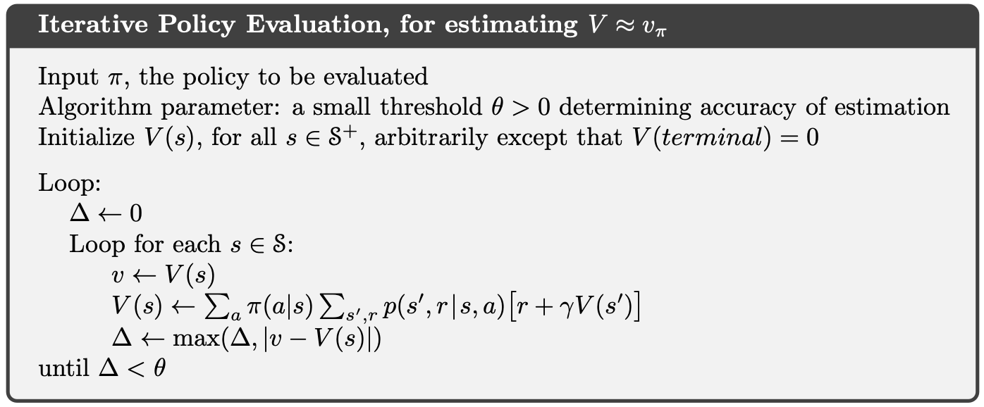
If the dynamics are known perfectly, this becomes a system of $|S|$ simultaneous linear equations in $|S|$ unknowns, where the unknowns are $v_\pi(s), s \in S$. If we consider an iterative sequence of value function approximations $v_0, v_1, v_2, \cdots,$ with initial approximation $v_0$ chosen arbitrarily e.g. $v_k(s) = 0 \; \forall s$ (ensuring terminal state = 0). We can update it using the Bellman equation:

$$\begin{gather*} v_{k+1}(s) = \sum_a \pi(a|s)\sum_{s',r} p(s',r|s,a)\Big [r+\gamma v_k(s')\Big ], \forall s \in S. \end{gather*}$$

Eventually this update will converge when $v_k = v_\pi$ after infinite sweeps of the state-space, the value function for our policy. This algorithm is called iterative policy evaluation. We call this update an expected update because it is based on the expectation over all possible next states, rather than a sample of reward/value from the next state. We think of the updates occurring through sweeps of state space.

Pseudocode

My code

• A typed version of my Code
• View my Code on Github

Policy Improvement

We can obtain a value function for an arbitrary policy $\pi$ as per the policy evaluation algorithm discussed above. We may then want to know if there is a policy $\pi'$ that is better than our current policy. A way of evaluating this is by taking a new action $a$ in state $s$ that is not in our current policy, running our policy thereafter and seeing how the value function changes. Formally that looks like:

$$\begin{gather*} q_\pi(s, a) \doteq \sum_{s',r} p(s',r|s,a)[r+\gamma v_\pi(s')]. \end{gather*}$$

Note the mixing of action-value and state-value functions. If taking this new action in state $s$ produces a value function that is greater than or equal to the previous value function for all states then we say the policy $\pi'$ is an improvement over $\pi$:

$$\begin{gather*} v_{\pi'}(s) \ge v_\pi(s),\forall s \in S. \end{gather*}$$

This is known as the policy improvement theorem. Critically, the value function must be greater than the previous value function for all states. One way of choosing new actions for policy improvement is by acting greedily w.r.t the value function. Acting greedily will always produce a new policy $\pi' \ge \pi$, but it is not necessarily the optimal policy immediately.

Policy Iteration

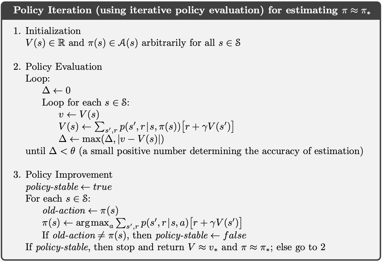
Once a policy, $\pi$, has been improved using $v_\pi$ to yield a better policy, $\pi'$, we can then compute $v_{\pi'}$ and improve it again to yield an even better $\pi''$. We can thus obtain a sequence of monotonically improving policies and value functions:

$$\begin{gather*} \pi_0 \xrightarrow{E} v_{\pi_0} \xrightarrow{I} \pi_1 \xrightarrow{E} v_{\pi_1} \xrightarrow{I} \pi_2 \xrightarrow{E} \cdots \xrightarrow{I} \pi_* \xrightarrow{E} v_*, \end{gather*}$$

where $\xrightarrow{E}$ denotes a policy evaluation and $\xrightarrow{I}$ denotes a policy improvement.

Pseudocode

My Code

• A typed version of my Code
• View my Code on Github

Value Iteration

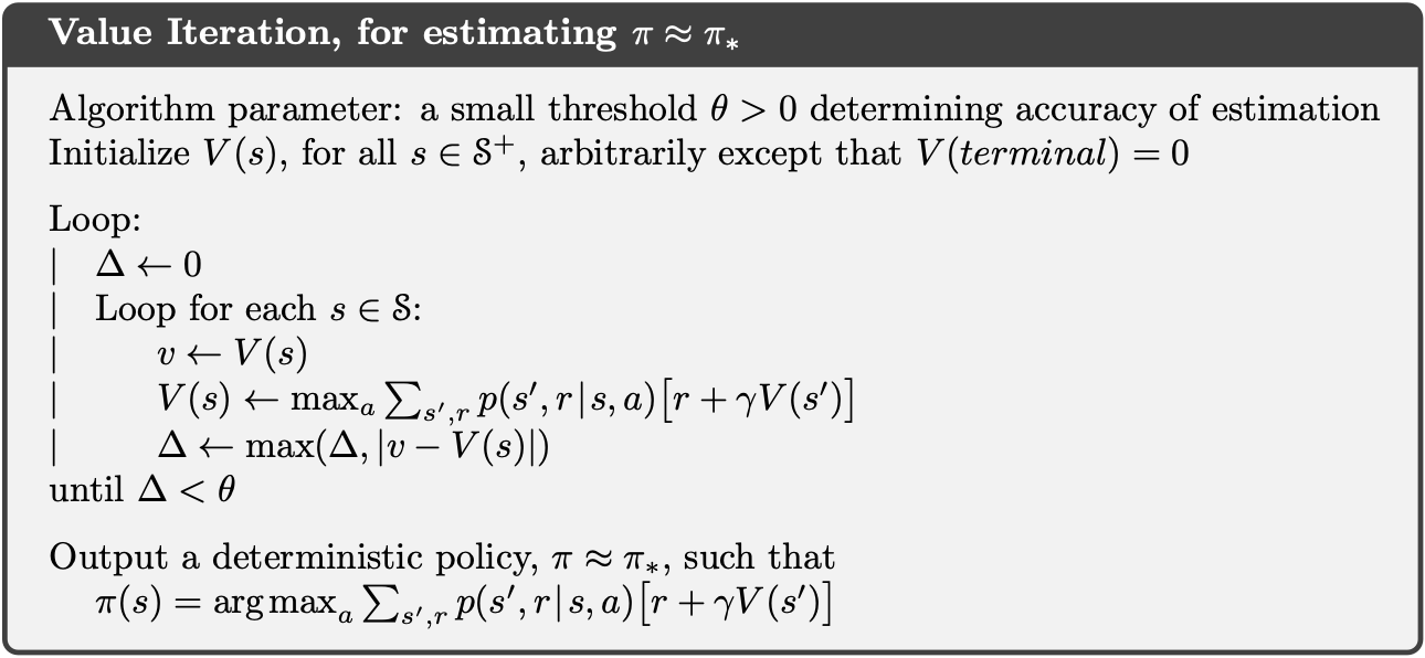
Above, we discussed policy iteration which requires full policy evaluation at each iteration step, an often expensive process which (formally) requires infinite sweeps of the state space to approach the true value function. In value iteration, the policy evaluation is stopped after one visit to each $s \in S$, or one sweep of the state space. Value iteration is achieved by turning the Bellman optimality equation into an update rule:

$$\begin{align*} v_{k+1}(s) & \doteq \max_{a} \mathbb{E}[R_{t+1}+\gamma v_k(S_{t+1})|S_t=s,A_t=a] \\ & = \max_{a} \sum_{s',r}p(s',r|s,a)[r+\gamma v_k(s')],\forall s \in S. \end{align*}$$

Value iteration effectively combines, in each of its sweeps, one sweep of policy evaluation and one sweep of policy improvement.

Pseudocode

My Code

• A typed version of my Code
• View my Code on Github

Synchronous Dynamic Programming Algorithms Summary

Problem	Bellman Equation	Algorithm
Prediction	Expectation Equation	Iterative Policy Evaluation
Control	Expectation Equation + Greedy Policy Improvement	Policy Iteration
Control	Optimality Equation	Value Iteration

• These algorithms are based on state-value functions $v_{\pi}(s)$ or $v_{*}(s)$
• Complexity $O(mn^2)$ per iteration, for m actions and n states
• The algorithms can also be applied to action-value functions $q_{\pi}(s,a)$ or $q_{*}(s,a)$
• Complexity $O(m^2 n^2)$ per iteration

Extensions to Dynamic Programming

Asynchronous Dynamic Programming

• Instead of backing up all states in parallel, we can pick any state to be the root of the backup and plugin the new value functions for the next iterations
• Reduced computation and guaranteed convergence if all the states are selected at least sometimes
• Three simple ideas
  • In-place dynamic programming
  • Prioritized sweeping
  • Real-time dynamic programming

In-place dynamic programming

• Synchronous value iteration stores two copies of the value function, old of the leaves and the new of the root state, for all $s \in S$

  $$\begin{gather*} v_{new}(s) \leftarrow \max_{a \in A} (R_s^a + \gamma \sum_{s' \in S} P^a_{ss^{'}} v_{old}(s^{'})) \\ v_{old} \leftarrow v_{new} \end{gather*}$$

• In-place value iteration only stores one copy of the value function, for all $s \in S$

  $$\begin{gather*} v(s) \leftarrow \max_{a \in A} (R_s^a + \gamma \sum_{s' \in S} P^a_{ss'} v(s')) \end{gather*}$$
  • We are going to plugin the latest value
  • The most important thing is how to order the states so as to compute things in the most efficient way
  • The ordering of the states really matters

Prioritized Sweeping

• A measure of how important it is to update any state in the MDPs
• Keep a priority queue to look at which state it is better to be updated
• Use the magnitude of Bellman error to guide state selection
• Backup the state with the largest remaining bellman error
• Update the bellman error of the affected states after each backup
• This requires knowledge of the reverse dynamics of the MDP i.e. predecessor states

Real-time Dynamic Programming

• Idea: Select the states that the agent is visiting
• Collect real samples from the agent's experience to guide the selection of states and update those samples
• After each time-step $S_t, A_t, R_{t+1}$
• Backup the state $S_t$
  $$\begin{gather*} v(S_t) \leftarrow \max_{a \in A} (R_{S_t}^a + \gamma \sum_{s' \in S} P^a_{S_ts'}v(s')) \end{gather*}$$
  ms in the field of reinforcement learning.

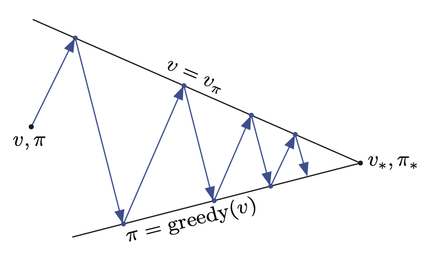
Generalized Policy Iteration

We use the term generalized policy iteration (GPI) to refer to the general idea of letting policy-evaluation and policy-improvement processes interact, independent of the granularity and other details of the two processes. Almost all reinforcement learning methods are well described as GPI. That is, all have identifiable policies and value functions, with the policy always being improved with respect to the value function and the value function always being driven toward the value function for the policy, as suggested by the diagram to the right. If both the evaluation process and the improvement process stabilize, that is, no longer produce changes, then the value function and policy must be optimal. The value function stabilizes only when it is consistent with the current policy, and the policy stabilizes only when it is greedy with respect to the current value function. Thus, both processes stabilize only when a policy has been found that is greedy with respect to its own evaluation function. This implies that the Bellman optimality equation holds, and thus that the policy and the value function are optimal.